How To Create A Neural Network From Scratch Using Python and Numpy

This will walk you through how to make a very simple neutal network with 3 layers without the implementation of biases.

Well I'd first like to go through the math and the algorithms behind the actual neural network before doing the code.

Mathematically speaking we can look at a neural network as a set of matrices of randomly initialized weights that we adjust according to how wrong the multiplication of our inputs and activation layers with our weight matrices are compared to the output.

Forward propogation is simply the multriplication of our inputs with our weights and back propagation is the adjustment.

So lets first look at forward propogation. Let the input layer be x, activation layers be a_i (multiple activation layers, we will index them with i) and the weights that correspond to each activation layer be W_i and lets just call the output layer y'.

For the sake of ease lets look at a simple visualization for a 3 layer neural network, and I find this visualization more helpful than the usual one with tons of arrows and I'll explain why.

 

With this visualization its more clear what exactly we are doing. We treat x, a_i and y' as vectors. We start with x and to get the next layers value, in this case a₁ we multiply by the weight matrix that corresponds to that layer which in this case is W₁ and then we repeat with W₂ and a₁ to get output layers value. Thus when initializing your neural network you need to be very careful of the size. For matrices we can only multiply a matrix A with matrix B if matrix A has the same number of columns as matrix B has rows. If that sounds confusing, let matrix A have n rows and m columns (we will call this an nxm matrix) B can only be multiplied with A if it has m rows and p columns (an mxp matrix). The resulting multiplication results in an nxp matrix, (nxm * mxp = nxp, the two equal numbers in the middle sorta "cancel out"). Since your input vector will be a nx1 matrix (column vector), we need our matrix of size mxn since our activation layer has m elements and as shown, a mxn * nx1 will result in a mx1 matrix or a column vector. If you work with a row vector instead, as in x = [x₁, ..., x_n] just flip the multiplication order and the size of the matrix, i.e a 1xn matrix multiplies with a nxm matrix to get an 1xm row vector. Or mathematically:

More generally:

In this case l_p is the layer we are starting from and l_p+1 is the next layer we want to find values for.

The next step to this is we want to apply our activation function to our neural network. There are many activation functions but the three that ill describe are sigmoid, tanh and ReLU. For this tutorial we are using sigmoid, but I will breifly describe the others as well. When applying any of these activation functions to a vector just apply the equation to every element in the vector. You can see a very thorough list here. 

Sigmoid:
Equation:

Graph:

This function brings higher negative values closer to zeros and higher positive values closer to one, which is effective for classification type problems. This graph approaches 1 as x approaches infinity and approaches 0 as x approaches negative inifinity.

Tanh:
Equation:

Graph:

This function is similar to sigmoid, except it brings higher negative values to -1 instead of 0.

ReLU:
Equation:

Graph: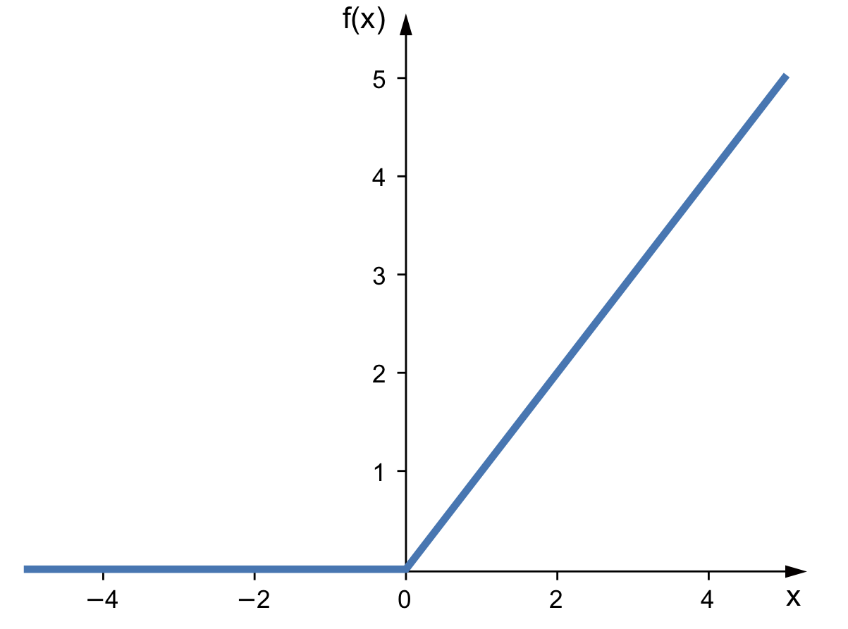

Thus when we translate to code our forward propogation function simply becomes:

• def forward(self, input_layer):
  	self.hidden_layer_1 = input_layer.dot(self.weights[0])
  	self.hidden_layer_1 = g(self.hidden_layer_1)
  	self.output_layer = self.hidden_layer_1.dot(self.weights[1])
  	self.output_layer = g(self.output_layer)
  

In this case since we are using sigmoid activation, our function g(x) becomes:

• from scipy.special import expit
  def g(v):
  	return expit(v)

Now, back propagation is a bit more tricky. Back propagation is the reverse of forward propagation. We are starting with the output we got y' and comparing it with our desired output y. We then take this difference and find out the cost of our current weights (i.e how wrong we are because of our current weights). Back propagation aims to minimize this cost. To begin with let us first define some key elements.

First lets define a term delta to calculate error in layer i as:

Where the '*' is the element wise multiplication of the previous layers error with the derivative of our activation function evaluated at the previous activation layer. And suppose we have s layers, our first delta term becomes

.

You start with this and begin finding the deltas of each layer (ignoring the input layer of course). Once you have those, calculate another delta, this one tells us by how much we need to change our weight matrix by. We will define it as:

Wher i is the ith layer and we are taking the error of the layer that comes after and after finding its matrix multiplication with activation layer i we have the amount we must change our W_i by.

So for our situation, we have a 3 layer network. Thus the steps become:
Find the layer deltas:

Find the weight deltas:

Where x is the input layer.

Now adjust the weights with the corresponding deltas:

Now translating all that into code, we get:

• def backward(self, x_train, y_train):
  	output_error = y_train - self.output_layer
  	del_out = output_error*g_prime(self.output_layer)
  	del_hl = output_error.dot(self.weights[1].T)*g_prime(self.hidden_layer_1)
  	self.weights[0] += self.lr*x_train.reshape(5,1).dot(del_hl.reshape(1,4))
  	self.weights[1] += self.lr*self.hidden_layer_1.reshape(4,1).dot(del_out.reshape(1, 3))

 Now we are done. To implement these I suggest making a neural network object with the __init__ initializing the random weights and setting sizes as well.

The next thing to look at is the current cost of your neural network. Looking at the cost is really helpful in debugging and fixing any errors. One such way of looking at error is using mean squared error, or MSE.

The formula is this:

When implementing it with your neural network itll be something like:

• def cost(self, y_train):
  	MSE = (np.square(self.output_layer - y_train))
  	return (1/self.s1)*np.sum(MSE)

Now to put everything together, out neural network object now becomes:

• class NN:
  
  	s1 = 0
  	s2 = 0
  	s3 = 0
  	lr = 0
  	weights = []
  	hidden_layer_1 = []
  	output_layer = []
  
  	def __init__(self, s1, s2, s3, lr):
  		self.s1 = s1
  		self.s2 = s2
  		self.s3 = s3
  		self.lr = lr
  		self.weights.append(np.random.rand(s1, s2))
  		self.weights.append(np.random.rand(s2, s3))
  
  	def forward(self, input_layer):
  		self.hidden_layer_1 = input_layer.dot(self.weights[0])
  		self.hidden_layer_1 = g(self.hidden_layer_1)
  		self.output_layer = self.hidden_layer_1.dot(self.weights[1])
  		self.output_layer = g(self.output_layer)
  
  	def backward(self, x_train, y_train):
  		output_error = y_train - self.output_layer
  		del_out = output_error*g_prime(self.output_layer)
  		del_hl = output_error.dot(self.weights[1].T)*g_prime(self.hidden_layer_1).reshape(1,4)
  		self.weights[0] += self.lr*x_train.reshape(5,1).dot(del_hl.reshape(1,4))
  		self.weights[1] += self.lr*self.hidden_layer_1.reshape(4,1).dot(del_out.reshape(1, 3))
  
  	def cost(self, y_train):
  		MSE = (np.square(self.output_layer - y_train))
  		return (1/self.s1)*np.sum(MSE)
  

Here you might find the variable lr, that is the learning rate. This helps the weights converge faster.

When running the neural network with our iris dataset, we must first start with regularizing our data and then making a train/test split. This is easily done with sklearns preprocessing library. Using it we end up with:

• data = datasets.load_iris()
  
  scaler = StandardScaler()
  lb = LabelBinarizer()
  
  x_train, x_test, y_train, y_test = train_test_split(data.data, data.target, test_size=0.33, random_state=42)
  
  x_train = scaler.fit_transform(x_train)
  x_test = scaler.transform(x_test)
  
  y_train = lb.fit_transform(y_train)
  y_test = lb.transform(y_test)

Then to initalize our neural net all we need to do is:

• net = NN(5,4,3,3)

Since our input layer is 5 and we have 3 different types of irises, the 5 at the beginning and the 3 that is the second to last number must stay that way. You can tinker with the hidden layer size 4, and the learning rate 3 to see which yields better results. The size 4 and learning rate 3 worked well for me though.

Now to actually train our dataset all we do is go forward, then backwards and then repeat. To get good results you should run the loop many times. I myself ran mine 1000 times whilst printing the cost. My cost ended up being 6.230206526533108e-6 which is very close to zero (although it isnt this everytime, sometimes higher sometimes lower).

Another thing to mention is that you won't have perfect one-hot vectors, so when testing your data give yourself a 0.1 or lower wiggle room. To make that more clear, floor anything below a 0.01 to zero and anything above a 0.9 to a 1. Thus the entire code now becomes:

• import numpy as np
  from sklearn import datasets
  import random
  from scipy.special import expit
  import matplotlib.pyplot as plt
  from sklearn.model_selection import train_test_split
  from sklearn.preprocessing import StandardScaler, LabelBinarizer
  from scipy.special import expit, logit
  
  #sigmoid
  def g(v):
  	return expit(v)
  
  def g_prime(v):
  	return v * (1 - v)
  
  class NN:
  
  	s1 = 0
  	s2 = 0
  	s3 = 0
  	lr = 0
  	weights = []
  	hidden_layer_1 = []
  	output_layer = []
  
  	def __init__(self, s1, s2, s3, lr):
  		self.s1 = s1
  		self.s2 = s2
  		self.s3 = s3
  		self.lr = lr
  		self.weights.append(np.random.rand(s1, s2))
  		self.weights.append(np.random.rand(s2, s3))
  
  	def forward(self, input_layer):
  		self.hidden_layer_1 = input_layer.dot(self.weights[0])
  		self.hidden_layer_1 = g(self.hidden_layer_1)
  		self.output_layer = self.hidden_layer_1.dot(self.weights[1])
  		self.output_layer = g(self.output_layer)
  
  	def backward(self, x_train, y_train):
  		output_error = y_train - self.output_layer
  		del_out = output_error*g_prime(self.output_layer)
  		del_hl = output_error.dot(self.weights[1].T)*g_prime(self.hidden_layer_1).reshape(1,4)
  		self.weights[0] += self.lr*x_train.reshape(5,1).dot(del_hl.reshape(1,4))
  		self.weights[1] += self.lr*self.hidden_layer_1.reshape(4,1).dot(del_out.reshape(1, 3))
  
  	def cost(self, y_train):
  		MSE = (np.square(self.output_layer - y_train))
  		return (1/self.s1)*np.sum(MSE)
  
  
  
  data = datasets.load_iris()
  
  scaler = StandardScaler()
  lb = LabelBinarizer()
  
  x_train, x_test, y_train, y_test = train_test_split(data.data, data.target, test_size=0.33, random_state=42)
  
  x_train = scaler.fit_transform(x_train)
  x_test = scaler.transform(x_test)
  
  y_train = lb.fit_transform(y_train)
  y_test = lb.transform(y_test)
  
  net = NN(5,4,3,3)
  
  for i in range(1000):
  	for i in range(len(x_train)):
  		net.forward(np.insert(x_train[i], 0, 1))
  		net.backward(np.insert(x_train[i], 0, 1), y_train[i])
  		print(net.cost(y_train[i]))
  
  count = 0
  
  for i in range(len(x_test)):
  	net.forward(np.insert(x_test[i], 0, 1))
  	hypothesis = net.output_layer
  	for j in range(len(hypothesis)):
  		if hypothesis[j] <= 0.01:
  			hypothesis[j] = 0
  		elif hypothesis[j] >= 0.9:
  			hypothesis[j] = 1
  	if np.array_equal(np.array(hypothesis), y_test[i]):
  		count+= 1	
  
  print(count/len(x_test))